Part 1: Data Exploration

Part 1: Data Exploration
Objective:
Import Python Packages:
Import & Clean Data:
PCA Analysis of the data:
References:

I completed the WQU Machine Learning course 3 months ago and wanted to explore some new challenges. As a result I am exploring this Kaggle competition for leisure and am following a website cited in the references.

Objective:

Predict house prices

Import Python Packages:

import pandas as pd
import matplotlib.pyplot as plt
import numpy as np
import seaborn as sb
import sklearn as sk

Import & Clean Data:

Two data sets are provided one for testing and the other for training.
We import each of the csv files into a pandas dataframe and remove any unwanted details

df_test = pd.read_csv('test.csv')
df_train = pd.read_csv('train.csv')
df_train.head()

	Id	MSSubClass	MSZoning	LotFrontage	LotArea	Street	Alley	LotShape	LandContour	Utilities	...	PoolQC	Fence	MiscFeature	MoSold	YrSold	SaleType	SaleCondition	SalePrice
0	1	60	RL	65.0	8450	Pave	NaN	Reg	Lvl	AllPub	...	NaN	NaN	NaN	2	2008	WD	Normal	208500
1	2	20	RL	80.0	9600	Pave	NaN	Reg	Lvl	AllPub	...	NaN	NaN	NaN	5	2007	WD	Normal	181500
2	3	60	RL	68.0	11250	Pave	NaN	IR1	Lvl	AllPub	...	NaN	NaN	NaN	9	2008	WD	Normal	223500
3	4	70	RL	60.0	9550	Pave	NaN	IR1	Lvl	AllPub	...	NaN	NaN	NaN	2	2006	WD	Abnorml	140000
4	5	60	RL	84.0	14260	Pave	NaN	IR1	Lvl	AllPub	...	NaN	NaN	NaN	12	2008	WD	Normal	250000

5 rows × 81 columns

print(df_train.shape)
print(df_test.shape)

(1460, 81)
(1459, 80)

Visualise the data

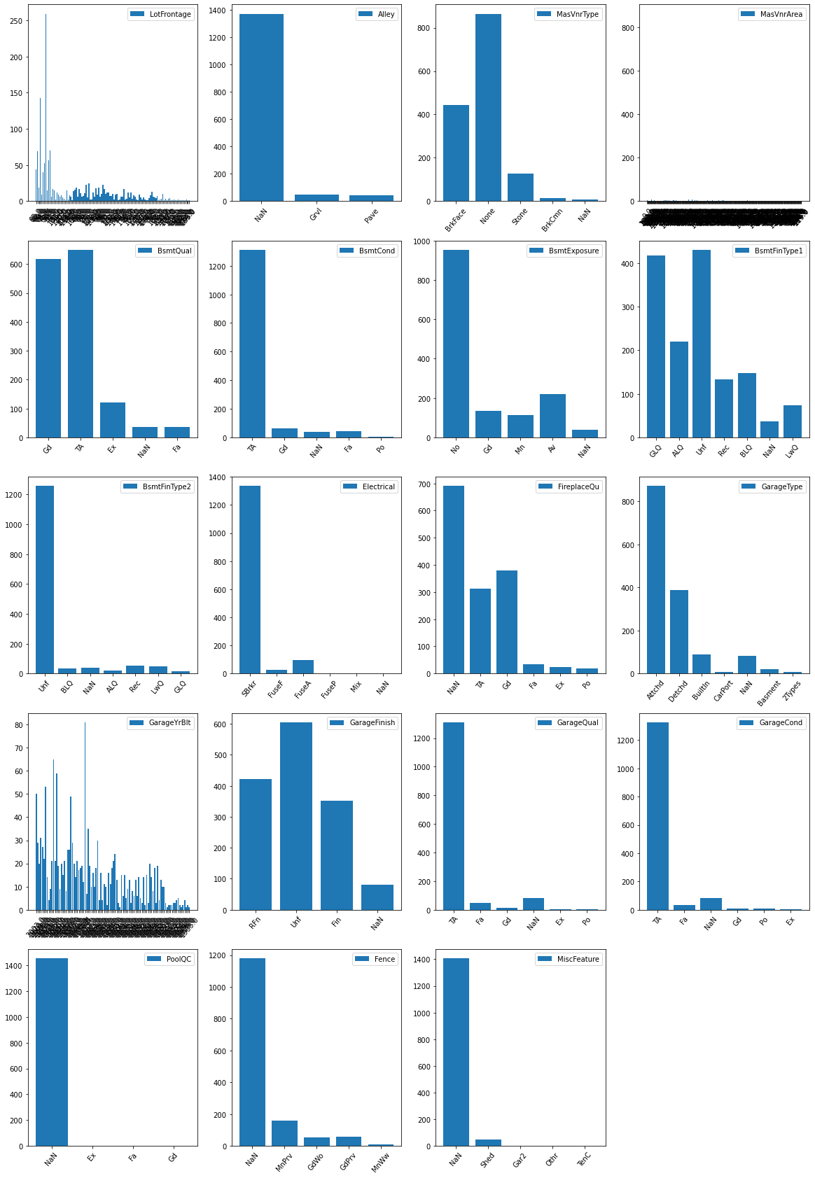
Apparently, the data has so many NaN data it may be wise not to drop them.
Below we use a simple function to determine all the unique entries in the columns with many NaN values
Since NaN is not a good key in a dictionary we will need to employ a work around for the possible NaN vales
We notice that for the following columns the ‘NaN’ values are too many and we do not expect them to contribute significantly to the ML algorithm:
- Alley
- FirePlace
- PoolQG
- Fence
- MiscFeture

def unique_tally(data):
    '''Returns a dictionary of the unique entries in a data column and their frequencies'''
    isnan = list(data.isnull())
    res = {}
    for i in range(len(data)):
        if isnan[i]:
            key_ = 'NaN'
        else:
            key_ = data[i]
        if key_ in res:
            res[key_] +=1
        else:
            res[key_] = 1
    return res

tallies = []
c = list(df_train.columns)
for col in c:
    tallies.append(unique_tally(df_train[col]))
indx =[]
for k in range(len(tallies)):
    if 'NaN' in tallies[k]:
        indx.append(k)
len(indx)
plt.figure(figsize= (20,30))
for i in range(len(indx)):
    plt.subplot(5,4,i+1)
    plt.bar(range(len(tallies[indx[i]])), list(tallies[indx[i]].values()), align='center', label = c[indx[i]])
    plt.xticks(range(len(tallies[indx[i]])), list(tallies[indx[i]].keys()), rotation=50)
    plt.legend()

png

# Analyse the test data in a similar way using Pandas functions
df_train.isnull().sum().sort_values(ascending=False)

PoolQC           1453
MiscFeature      1406
Alley            1369
Fence            1179
FireplaceQu       690
                 ... 
CentralAir          0
SaleCondition       0
Heating             0
TotalBsmtSF         0
Id                  0
Length: 81, dtype: int64

# Analyse the test data in a similar way using Pandas functions
df_test.isnull().sum().sort_values(ascending=False)

PoolQC         1456
MiscFeature    1408
Alley          1352
Fence          1169
FireplaceQu     730
               ... 
Electrical        0
CentralAir        0
HeatingQC         0
Foundation        0
Id                0
Length: 80, dtype: int64

So we will drop the following columns since they have more than 50% ‘NaN’ data values
- PoolQC
- MiscFeature
- Alley
- Fence
Also, we will drop the ‘Id’ column as it is irrelevant to the calculations

df_train1 = df_train.drop(['Id', 'PoolQC', 'MiscFeature', 'Alley', 'Fence'], axis = 1)
df_test1 = df_test.drop(['Id', 'PoolQC', 'MiscFeature', 'Alley', 'Fence'], axis = 1)

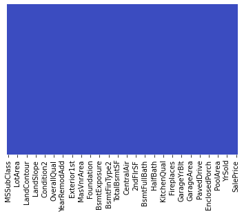
Replacing NaN Values:

Clearly, not all ‘NaN’ values need to be discarded.
The data columns have various data types and we need to replace the these missing values in a consistent manner
We do this for both the test and training data
We will replace ‘NaN’ values depending on some conditions as follows:
- If the data in the column is numerical replace NaN with the mean
- If the data in the column is of string type, replace NaN with modal category
We proceed as follows:

def replace_nan(df):
    col = 0
    c = list(df.columns)
    for i in df.dtypes:
        if i in [np.int64, np.float64]:
            df[c[col]]=df[c[col]].fillna(df[c[col]].mean())        
        elif i == object:
            df[c[col]]=df[c[col]].fillna(df[c[col]].mode()[0])
        col+=1

replace_nan(df_train1)
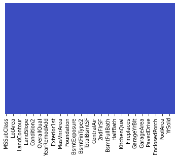
replace_nan(df_test1)

sb.heatmap(df_train1.isnull(),yticklabels=False,cbar=False,cmap='coolwarm')

png

sb.heatmap(df_test1.isnull(),yticklabels=False,cbar=False,cmap='coolwarm')

png

Convert Categorical Data:

All categorical data needs to be converted into numerical categories
This will enable the algorithms to understand the data

def category_to_num(df):
    '''Takes in a column of data and determines how many unique vakues there are
        Each value is assigned a unique natural number & the data is updated
        Returns the categories.'''
    categs = sorted(list(df_train1[col[ci]].unique()))
    for num in range(len(categs)):
        df.loc[df==categs[num]] = num
    return categs

ci = 0
col = list(df_train1.columns)
categ = {}
for dt in df_train1.dtypes:
    if dt == object:
        categs= category_to_num(df_train1[col[ci]])
        categ[col[ci]] = categs
    ci+=1
df_train1.head()

C:\Users\zmakumbe\.conda\envs\wqu_ml_fin\lib\site-packages\pandas\core\indexing.py:670: SettingWithCopyWarning: 
A value is trying to be set on a copy of a slice from a DataFrame

See the caveats in the documentation: https://pandas.pydata.org/pandas-docs/stable/user_guide/indexing.html#returning-a-view-versus-a-copy
  iloc._setitem_with_indexer(indexer, value)

	MSSubClass	MSZoning	LotFrontage	LotArea	Street	LotShape	LandContour	LotConfig	...	EnclosedPorch	MoSold	YrSold	SaleType	SaleCondition	SalePrice
0	60	3	65.0	8450	1	3	3	4	...	0	2	2008	8	4	208500
1	20	3	80.0	9600	1	3	3	2	...	0	5	2007	8	4	181500
2	60	3	68.0	11250	1	0	3	4	...	0	9	2008	8	4	223500
3	70	3	60.0	9550	1	0	3	0	...	272	2	2006	8	0	140000
4	60	3	84.0	14260	1	0	3	2	...	0	12	2008	8	4	250000

5 rows × 76 columns

ci = 0
col = list(df_test1.columns)
categ = {}
for dt in df_test1.dtypes:
    if dt == object:
        categs= category_to_num(df_test1[col[ci]])
        categ[col[ci]] = categs
    ci+=1

plt.figure(figsize=(10,5))
y = df_train.SalePrice
sb.set_style('whitegrid')
plt.subplot(121)
sb.distplot(y)

df_train['SalePrice_log'] = np.log(df_train.SalePrice)
y2 = df_train.SalePrice_log
plt.subplot(122)
sb.distplot(y2)
plt.show()

C:\Users\zmakumbe\.conda\envs\wqu_ml_fin\lib\site-packages\seaborn\distributions.py:2557: FutureWarning: `distplot` is a deprecated function and will be removed in a future version. Please adapt your code to use either `displot` (a figure-level function with similar flexibility) or `histplot` (an axes-level function for histograms).
  warnings.warn(msg, FutureWarning)
C:\Users\zmakumbe\.conda\envs\wqu_ml_fin\lib\site-packages\seaborn\distributions.py:2557: FutureWarning: `distplot` is a deprecated function and will be removed in a future version. Please adapt your code to use either `displot` (a figure-level function with similar flexibility) or `histplot` (an axes-level function for histograms).
  warnings.warn(msg, FutureWarning)

png

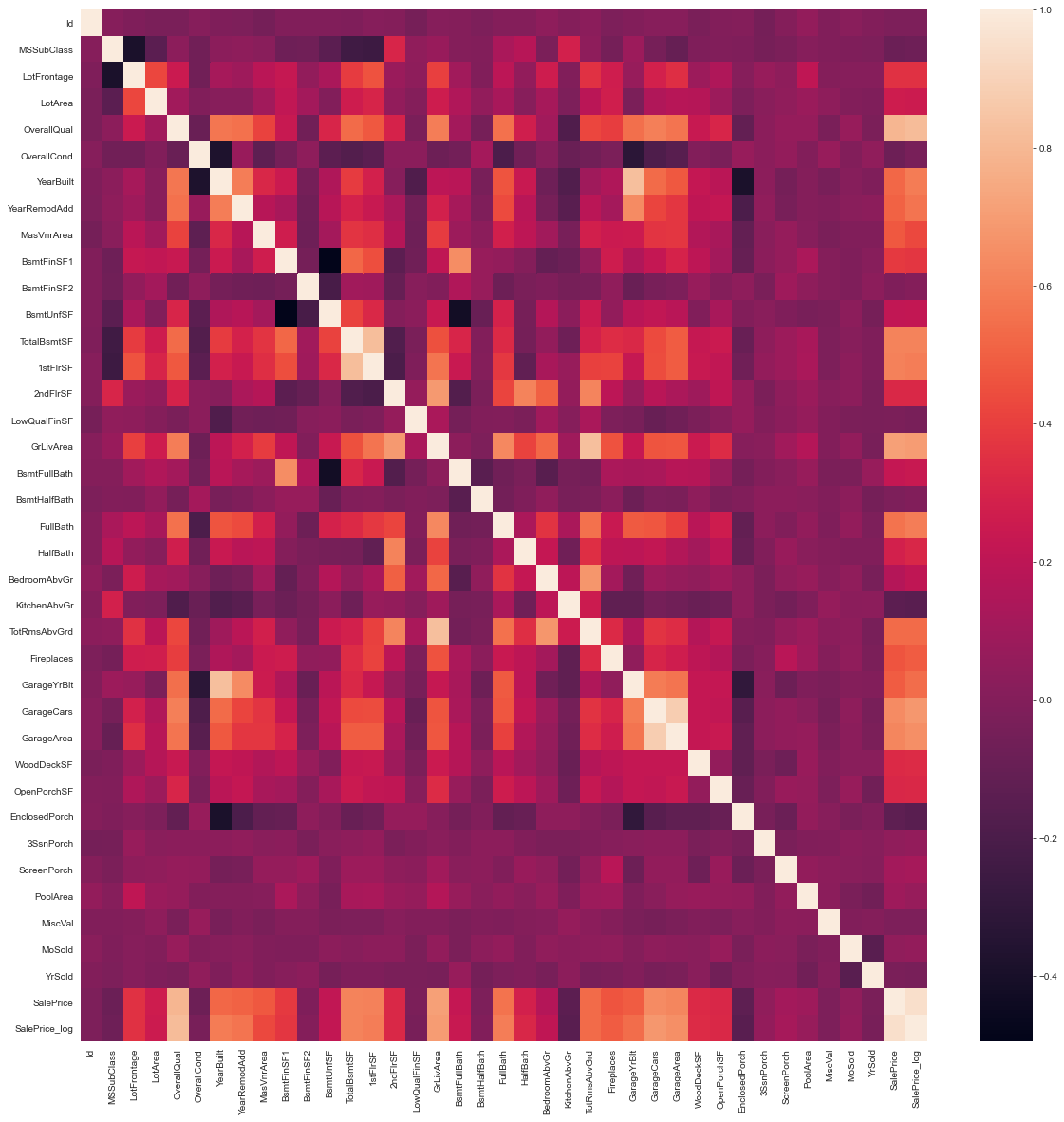
Data Correlation:

It is important to determine any interdependencies if they exist.

# Lets explore the correlations in our data set 
plt.figure(figsize=(20,20))
sb.heatmap(df_train.corr())

<AxesSubplot:>

png

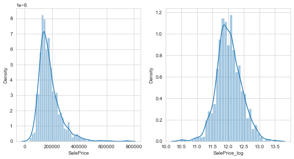
Visualising the output data

Next, taking the Sale Price data (which will bo our output variable) we plot a bar graph
From above, we find that the data is skewed but the log-transoformed data has a much better distribution
Such transformations help us avoid having to remove outliers.

PCA Analysis of the data:

Considering how many columns we have as well as the hunch we have pertaining to the ‘NaN’ values, we expect some columns to be redundant
We conduct a Principal Component Analysis (PCA) in order to determine if a smaller set of the data can be used to determine the output

from sklearn.model_selection import train_test_split 
from sklearn.linear_model import LinearRegression
from sklearn.decomposition import PCA 
from sklearn.preprocessing import StandardScaler 

#Setting the input and output variables
x = df_train1[c[:-1]]
y = df_train1['SalePrice']

#Splitting the data into training and testing data for a trial run
X_train, X_test, y_train, y_test = train_test_split(x, y, test_size = 0.2, random_state = 0)

sc = StandardScaler()

X_train = sc.fit_transform(X_train) 
X_test = sc.transform(X_test) 
# Applying PCA function on training 
# and testing set of X component 
  
pca = PCA(n_components = 50) 
  
X_train = pca.fit_transform(X_train) 
X_test = pca.transform(X_test) 
  
explained_variance = pca.explained_variance_ratio_
print('%-age of variance explained by the 45 principal components')
np.round(explained_variance*100,1)

%-age of variance explained by the 45 principal components

array([13.7,  5.6,  4.9,  4. ,  3. ,  2.8,  2.4,  2.3,  2.2,  2.1,  2. ,
        2. ,  1.9,  1.8,  1.7,  1.6,  1.6,  1.6,  1.5,  1.5,  1.5,  1.5,
        1.4,  1.4,  1.4,  1.3,  1.3,  1.2,  1.2,  1.2,  1.2,  1.1,  1.1,
        1.1,  1. ,  1. ,  1. ,  0.9,  0.9,  0.9,  0.9,  0.8,  0.8,  0.8,
        0.8,  0.7,  0.7,  0.7,  0.7,  0.7])

plt.figure(figsize=(10,5))
plt.plot(np.cumsum(pca.explained_variance_ratio_) )
plt.xticks(np.arange(start=0, stop=len(pca.explained_variance_ratio_), step=1),rotation = 70)
plt.grid()
plt.show()

png

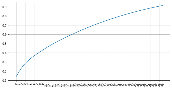
After conducting the PCA analysis we find that we need at least
- 35 data columns to explain at least 80% of the variation in the data,
- 40 data columns to explain at least 85% of the variation in the data, and
- 47 data columns to explain at least 90% of the variation in the data

# Create linear regression object 
regr = LinearRegression() 
# Fit 
regr.fit(X_train, y_train) 
# Calibration 
regr.score(X_test, y_test)

0.6565305727301065

pca = PCA(n_components = 50) 

regr_pca = LinearRegression() 

# Fit 
X_pca_train = pca.fit_transform(X_train) 
X_pca_test = pca.fit_transform(X_test) 

regr_pca.fit(X_pca_train, y_train) 
regr.score(X_pca_test, y_test)
#cross_val_score(regr_pca, X_pca_train, y_train).mean()

-1.0756078955375763

References:

https://www.educative.io/edpresso/how-to-check-if-a-key-exists-in-a-python-dictionary
https://towardsdatascience.com/predicting-house-prices-with-machine-learning-62d5bcd0d68f