Risk Management: VAR and CVA
We want to find ways of objectively quantifying risk. We will discuss two kinds of risk management tools
- Value at Risk (VaR)
- Credit Valuation adjustment (CVA)
Some Definitions:
Risk Metric:
A technique to measure and quantify risk in a portfolio.
Portfolio
A group of assets
Examples of Risk Metrics
- Volatility (variance)
- Correlation
These give us a sense of how much a portfolio could reduce and how susceptible it is to wild swings. However, the assumption is that the underlying distribution is multi-variate normal. This is not a practical assumption though. Hence, we need more general metrics at our disposal.
VaR
Value at risk (VaR) is a measure of how much our portfolio stands to lose at a given probability and within a specified time frame It can be given in absolute (dollar) terms or as a percentage of the portfolio value. Let our current portfolio value be given as $X(t)$. Then the return on the portfolio is given by \(R_{t,T}=\frac{X(T+t)-X(t)}{X(t)}.\)
Let the $\alpha$ quantile of the returns be given by \(\mathbb{P}(R_{t,T}<x_{\alpha}(t,T))=\alpha.\)
VaR is then defined as \(VaR_{\alpha}=\Big\{^{-x_{\alpha}(t,T)\text{ when looking at returns}}_{x_{\alpha}(t,T)X(t) \text{ when looking at portfolio vlue}}\)
Computing Var:
The two methods we will consider are
- Monte Carlo VaR
- Historical VaR
Monte Carlo VaR
Here we use simulation methods to project/produce possible asset values and get a feel of what would happen to our portfolio. In order to employ Monte Carlo we need to
- Determine the statistical behaviour of our assets of interest
- Simulate possible trajectories/terminal values of each asset
- Compute the total portfolio value
- Find the $\alpha$-quantile of the simulated prtfolio
Historical VaR
No assumption is made as to the underlying distribution of the asset. Only the available historical data is use to extrapolate what could happen to the assets and hence to the portfolio. Historical VaR assumes that:
- Past behaviour of the assets is determines what happens in the future
- Similarly, it assumes that the prevailing conditions of the past will remain as they are.
In computing Historical VaR
- Obtain historical data for each asset in the portfolio
- Compute each asset return
- Randomly sample a specific subset of returns for each asset
- Compute portfolio value for each possible scenario
- Find the $\alpha$-quantile of the projected prtfolio
A Computation Example
Please follow the comments in the code below
import numpy as np
from scipy.stats import norm
import numpy.matlib
import matplotlib.pyplot as plt
import math
import random
Monte Carlo:
#Create fictitious data with the parameters given below

S0=np.array([[100], [95], [50]])
sigm=np.array([[0.15], [0.2], [0.3]])
cor_mat=np.array([[1, 0.2, 0.4], [0.2, 1, 0.8], [0.4, 0.8, 1]])
L=np.linalg.cholesky(cor_mat)
r=0.1
T=1
#Assume that we hold one unit of each asset
#Lets compute the value of the portfolio

np.random.seed(0)
num_realisations=10000
alpha = 0.05

#Current portfolio value
portfolio_val_curr=np.sum(S0)
#We will assume that each asset follows a Geometric Brownian Motion and the below function describes that:

def terminal_share_prices(S_0,risk_free_int,sigma,Z,T):
    '''Geometric Brownian Motion'''
    return S_0*np.exp((risk_free_int-0.5*sigma**2)*T+sigma*np.sqrt(T)*Z)
#Now we go on to cumpute the actual simulations
#Compute 10000 realisations for the future portfolio values

Z=np.matmul(L,norm.rvs(size=[3,num_realisations]))
portfolio_fut_vl=np.sum(terminal_share_prices(S0,r,sigm,Z,T),axis=0)
#We will compute the compute the porfolio returns
portfolio_ret=(portfolio_fut_vl-portfolio_val_curr)/portfolio_val_curr

#In order to compute the percentiles we need to sort the returns
portfolio_ret=np.sort(portfolio_ret)

#To compute VaR
mVaR_appx=portfolio_ret[int (np.floor(alpha*num_realisations))-1]
Historical VaR:
#Import the extra needed libraries
from scipy.stats import uniform
def share_path(S_0,risk_free_int,sigma,Z,dT):
    '''Generates price paths'''
    return S_0*np.exp(np.cumsum((risk_free_int-0.5*sigm*sigm)*dT+sigm*np.matlib.transpose(Z)*np.sqrt(dT)))
#Obtaining synthetic historical data
np.random.seed(0)

#Obtain data for N years
n_Years = 3
T=n_Years*365
Z = norm.rvs(size = [3,n_Years*365])

num_samples = 10000
#One day at a time
dT=1

#Correlated Normal variables
corr_Z = np.transpose(np.matmul(L,Z))

#Computing the simulted price paths
price_path = share_path(S0,r,sigm,corr_Z,dT)
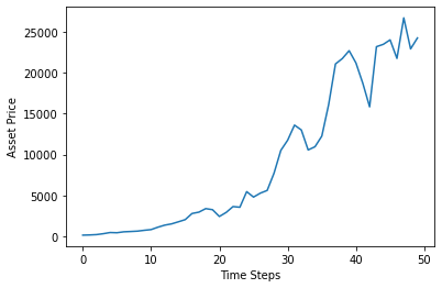
#Let us view one of the trajectories of the simulated price path
plt.plot(price_path[0][:50])
plt.xlabel('Time Steps')
plt.ylabel('Asset Price')
plt.show()

hist_S0=price_path[-1]
hist_port_val=np.sum(hist_S0)
hist_port_return=[None]*num_samples


#Comute the logarithm of each entry in the numpy array
log_returns_price=np.log(price_path)

#Compute the differences
log_returns_price = np.diff(log_returns_price,axis=1)
In oreder to have some randomness in our computations, we will randomly sample from the log returns of each asset by sampling from the uniform distribution on $[0,T]$. Recall that in the code $T$ is the total number of days.
for i in range(num_samples):
    rand_samp = uniform.rvs(size=365)*(len(price_path)-1)
    rand_samp = [int(x) for x in rand_samp]
    share_return_sampl = log_returns_price[rand_samp]
    s_term_sampl = S0*np.exp(np.sum(share_return_sampl,axis=1))
    hist_port_return[i]= (np.sum(s_term_sampl) - hist_port_val)/hist_port_val
CVA
When two financial entities enter into an agreement, there is a chance that one of them will fail to honor their agreement. This risk is called risk of default.
In addition, when trading shares or stock, the company itself can go bankrupt. For contracts traded at an exchanges, the excahnge ensures that the contracts are honored. However, for OTC (over the counter trading) there is a lot of exposure ot Counterparty credit risk or default risk.
How much is exposed? What are the chances of loss? How much does one stand to loose? Is there a chance of recovery?
These are questions answered in the study of credit risk models.
Terms:
- Exposure this is the amount you stand to loose \(V(t)=\max\{V(t),0\}\)
- Current exposure
- Expected Exposure
- Potential future exposure
Merton improved the Black-Scholes model to include the possibility of default which in it’s simplest form is that the value of the firm falls below a given threshold $D$ which can be thought of as the debt. In this situation the firm value is modelled by a Geometric Brownian Motion as” \(dV_t=rV_tdt+\sigma dW_t; \; V_0=v.\) It is further assumed that the debt is due at time $T$, hence default can only occur at that time. The debtors receive: \(\min\{V_T,D\}=D-(D-V_T)^+\) Thus the expected present value is given as: \(\mathbb{E}[e^{-rT}\min\{V_T,D\}]=De^{-rT}-P(V_0,r,\sigma,D,T)\) where \(P(V_0,r,\sigma,D,T)=V_0\Phi(-d_1)+(1-\Phi(-d_2))De^{-rT}\) is the Black-Scholes Put option price with $d_{1,2}$ defined as usual.
It is known that default occurs when the firm value falls below their debt. Thus the probability of defaul is given as: \(\mathbb{Q}[V_T<D]=\Phi(-d_2).\)
Portfolio CVA
It is possible that default can occur at any time. In general, we consider the time of default to be $\tau$, but in this discussion we will let $\tau = T$. Let $X_t$ be the value of the portfolio at time $t$ thus CVA is given as: \(CVA=\mathbb{E}[e^{-r\tau}(1-\delta)X_{\tau}\mathbb{1}_{\tau=T}=\mathbb{E}[e^{-rT}(1-\delta)X_{T}\mathbb{1}_{V_{T}<D}]\) A simple formula may be obtained in the case where the portfolio is independent of the firm value. On the other hand, we often notice some correlation between $X_t$ and $V_t$. This introduces the ida of right way and wrong way risk.
- Right way risk is when as the value of the portfolio increases the risk of default goes down. This comes about as a result of positive correlation.
- Wrong way risk is that as the value of the portfolio rises the risk of defaul rises too. A result of negative correlation.
Computational Example
#Assume that the above libraries have been loaded
risk_free = 0.1

S_0 = 100
sigma_Stock = 0.3

strike = 110
T = 1

#Firm values:
V_0 = 200
sigma_Firm = 0.25
debt = 180
recovery_rate = 0.2

num_steps = 10000

def call_pay_off(S_T, K):
    '''returns the pay off of a call option'''
    return np.maximum(S_T-K,0)

def CVA_Calculator(S0, sigma_S, V0, sigma_V, r, T, delta, D, corr, K, num_steps):
    if(corr == 1 or corr ==-1):
        norm_vector = norm.rvs(size = num_steps)
        norm_vector2 = corr*norm_vector
        corr_Z_matrix = np.array([norm_vector,norm_vector2])
    else:
        corr_matr = np.array([[1,corr],[corr,1]])
        norm_matr = norm.rvs(size = np.array([2,num_steps]))
        corr_Z_matrix = np.matmul(np.linalg.cholesky(corr_matr),norm_matr)

    S_T = terminal_share_prices(S0,risk_free,sigma_S,corr_Z_matrix[0,],T)
    call_val = call_pay_off(S_T, K)
    V_T = terminal_share_prices(V0,risk_free,sigma_V,corr_Z_matrix[1,],T)
    loss_val = np.exp(-r*T)*(1-delta)*(V_T<D)*call_val
    return np.mean(loss_val)
np.random.seed(0)

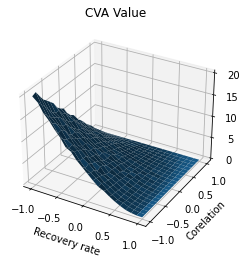
#We want to investigate the impact of the recovery rate on the CVA
recovery = np.linspace(-1,1,21)
correlation = np.linspace(-1,1,21)

CVA_Est = [None]*len(recovery)
CV_std = [None]*len(recovery)

#Lets compute CVA for each recovery rate

CVA = np.zeros((len(recovery),len(correlation)), dtype = np.float)
for i in range(len(recovery)):
    for j in range(len(correlation)):
        CVA[i,j]=CVA_Calculator(S_0, sigma_Stock, V_0, sigma_Firm, risk_free, T, recovery[i], debt, correlation[j], strike, num_steps)
#3D Plotting of the CVA surface
x, y = np.meshgrid(recovery, correlation)
fig = plt.figure()#figsize = (9,5)
ax = fig.gca(projection='3d')
plt.xlabel('Recovery rate')
plt.ylabel('Corelation')
plt.title('CVA Value')

# Plot the surface.
surf = ax.plot_surface(x, y, CVA)

plt.show()

References:
- Derivatives analytics with Python data analysis, models, simulation, calibration and hedging, Y. Hilpisch
- WQU
- matplotlib Website