Black Scoles Option Pricing
Having discussed Monte Carlo methods, we now want to p rice plain Vanilla options using Monte Carlo methods. These, however, do have cosed form solutions but we will use that to compare withe Monte Carlo (MC) solution
Model Introduction and assumptions
Asset Price Model
Let $(\Omega, \mathcal{F}, \mathbb{F}, \mathbb{P})$ be the filtered complete probability space describing our market. We consider $\mathbb{P}$ to be the market probability model. Under these conditions we assume that the stock price is described by the following stochastic differential equation (SDE): \(dS_t=S_t(\mu dt+\sigma dW_t)\) where
- $W=(W_t)_{t\geq 0}$ is standard Brownian Motion
- $\mu$ is the average return of the stock
- $\sigma$ is the standard deviation of the return otherwise known as volatility.
By making the market model as above, Black Scholes made some simplifying assumptions as below:
Model Assumptions
- There is a constant continuous risk free interest rate $r$.
- The market is frictionless. That is no transaction costs, default risk, spreads, taxes, and no dividends
- The market is completely liquid and short selling is allowed
- No arbitrage is possible
Pricing the Option
In order to satisfy the fourth assumption we need to find an equivalent martingale measure (EMM) $\mathbb{Q}$ such that the discunted asset price $\hat{S}_t=e^{-r(T-t)}S_T$ is a martingale. Thus under the risk neutral measure $\mathbb{Q}$ the dynamics of ${S}_t$ are as follows: \(dS_t=S_t(r dt+\sigma dW^{\mathbb{Q}}_t)\) where $W^{\mathbb{Q}}$ is the standard Brownian motion under ${\mathbb{Q}}$. By Ito formula, we find that
\[S_t=S_0\exp\Big((r-\frac{1}{2}\sigma^2) t+\sigma W^{\mathbb{Q}}_t\Big).\]Recall that $W_t~N(0,t)$ thus $W_t=Z\sqrt{t}$ where is $Z$ is a standard normal variate.
European Option
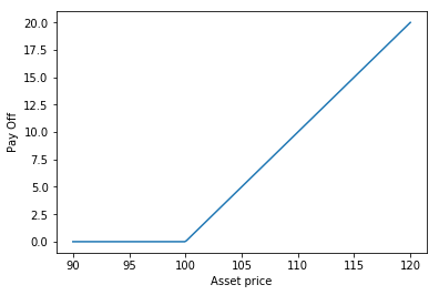
European option is a financial contract in which the holder has the right to purchase stock of a particular asset at a pre-specified price. The contract has a specific life span, expiration date, maturity or horizon. The holder will exercise the contract if the asset is higher than the prespecified price known as the strike price $K$. Otherwise the cotract expires worthless. Let the pay off $h$ be defined as follows: \(h(S_T)=(S_T-K)^+\)
import numpy as np
import matplotlib.pyplot as plt
import scipy.stats as sts
import math

def pay_off(s,k):
    if s>k:
        r=s-k
    else:
        r=0
    return r

K=100
S=np.linspace(90,120,200)
p=[]
for i in range(len(S)):
    p.append(pay_off(S[i],K))

plt.plot(S,p)
plt.xlabel("Asset price")
plt.ylabel("Pay Off")

Though the above implementation gets the job done, it is neither parsimonious, fast nor Pythonic. We can implement the vectorisation by using numpy arrays as follows:
def call_payoff(S,K):
    '''Computes the pay off given asset price S and strike K'''
    po=np.maximum(S-K,0)
    return po

def terminal_asset_val(int_rate, S0, sigm, T, norm_val):
    '''Computes the terminal stock price'''
    S_T=S0*np.exp((int_rate-0.5*sigm**2)*T+sigm*np.sqrt(T)*norm_val)
    return S_T
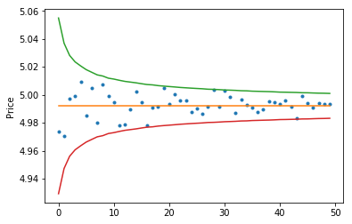
We can now iteraatively compute the option price by taking the mean of several estimates:
num_values =50 #Number of comutations
call_temp=[] #Create list of call price estimates
call_std=[] #Create list of call price std deviations

r=0.1 #risk free interest rate
sig=0.01 #standard dev of returns
T=1 #Option contract horizon
curr_tim=0
S0=100 #Initial asset price
K=105 #Strike price

for it in range(1,num_values+1):
    Z=sts.norm.rvs(size=it*1000)
    ST=terminal_asset_val(r,S0,sig,T-curr_tim,Z)
    p=np.exp(-r*T)*call_payoff(ST,K)
    call_temp.append(np.mean(p))
    call_std.append(np.std(p)/math.sqrt(it*1000))
Remark
For the sake of comparison, we will compute the analytic option price according to Black and Scholes. We know that, the option orice is given as \(\Pi=S_0\Phi(d_1)-e^{-rt}K\Phi(d_2)\) where $d_1=\frac{\ln(S_0/K)+(r+\sigma^2/2)(T-t)}{\sigma\sqrt{T-t}}$ and $d_2=d_1-\sigma\sqrt{T-t}.$
Each of the above formulas are represented by the Pythin functions below:
def d_pm(r,S0,sig,T,t,K,pm):
    '''Compute d_1 and d_2 in the Black Scholes option pricing model'''
    if pm==1:
        d=(np.log(S0/K)+(r+sig**2/2)*(T-t))/(sig*np.sqrt(T-t))
    else:
        d=d_pm(r,S0,sig,T,t,K,1)-sig*np.sqrt(T-t)
    return d

def Black_Scholes_Analytic(rate,S_0,sigm,Tt,tt,Kk):
    '''Compute the analytic Black Scholes option price'''
    d1=d_pm(rate,S_0,sigm,Tt,tt,Kk,1)
    d2=d_pm(rate,S_0,sigm,Tt,tt,Kk,-1)
    price = S_0*sts.norm.cdf(d1)-np.exp(-r*(Tt-tt))*Kk*sts.norm.cdf(d2)
    return price

#create an list of analytical option prices
analytic_p=[Black_Scholes_Analytic(r,S0,sig,T,curr_tim,K)]*num_values


#Let us visualise the mote carlo option pricing results against the analytic results

plt.plot(call_temp, '.')
plt.plot(analytic_p)
plt.plot(analytic_p+2*np.array(call_std))
plt.plot(analytic_p-2*np.array(call_std))
plt.ylabel("Price")
plt.show()

Conclusion
We used both an analytic and Monte Carlo approach to obtain the option price of a plain vanilla option in a Black-Scholes market